

Liberate and Elevate: Dynamic System Planning for a Grid That Delivers More
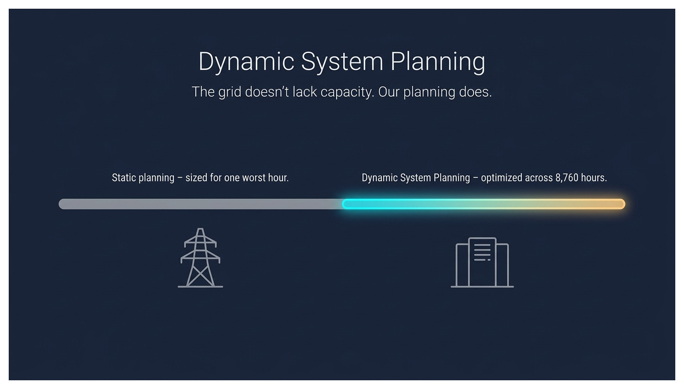
The grid doesn't lack capacity. Our planning does.

The Grid Is Under Unprecedented Interconnection Pressure
The US power system is facing an interconnection crisis on both sides of the meter. Data centers are projected to add a staggering 50 -90 GW of new electrical load by 2030. While these estimates vary widely and continue to be revised upward, the same trajectories are seen in Europe and the Asia-Pacific. The additional trends in electrification from transportation, manufacturing, and heating are making demand growth harder to anticipate for most grid planners. Much of this new load is inherently flexible: EV charging can shift off-peak hours, heat pumps and water heaters can pre-condition, and building HVAC systems can modulate in response to grid signals. What data centers offer at campus scale, these loads offer in aggregate. To add on top of that, generation and storage needed to serve this load (and meet decarbonization commitments) face the same bottleneck. For example, Berkeley Lab reports approximately 2,300 GW of generation and storage actively seeking interconnection as of year-end 2024, with average wait times exceeding four years. The physical grid infrastructure to connect either new loads or new supply simply does not exist yet.
Utilities and ISOs are all scrambling at the moment. We are seeing PJM Interconnection, ERCOT, Midcontinent Independent System Operator (MISO), and European TSOs all revising their peak load forecasts upward. This is astonishing as it’s the first time in decades that this is happening, and they’re flagging capacity adequacy as one of the concerns. The twin questions facing the industry are: “How do we connect massive new loads fast enough?” and “How do we connect the generation to serve them?” Both are stuck in the same queue, constrained by the same planning methodology.
The simple answer is to build more generation and transmission. While this is one approach, it’s dangerously incomplete. Average transmission projects take about 7-12 years when they start with planning ending in energization. In addition, new generation interconnection faces 5+ year queues in most RTOs. Supply chain constraints have pushed transmission capex well above pre-2020 baselines. Some components have even doubled in cost. The pipeline of data center demand will not wait for that long, though.
This paper proposes that the answer to the immediate crisis is already in front of us. The existing grid has far more capacity than we use, if we plan for it differently. We call this approach Dynamic System Planning.
The stakes are concrete. If Dynamic System Planning (DSP) were implemented across constrained US transmission corridors, preliminary analysis suggests it could unlock 100-150 GW of additional effective interconnection capacity from existing infrastructure, compress interconnection timelines by 3-7 years for qualifying projects, and avoid or defer $30-60 billion in new transmission investment. These are not theoretical ceilings. They are engineering estimates derived from the capacity headroom that dynamic ratings reveal (typically 20-40% above static ratings for the majority of hours), the demand-side flexibility that data center and generation operators can credibly provide, and the cost differentials between DSP portfolio solutions and conventional new-build alternatives. The methodology behind these figures is outlined in the Path Forward section; the numbers will sharpen as pilot data becomes available.
The Problem: A Grid Sized for One Hour
The core problem is not that the grid is too small; it’s that the grid is planned around the wrong conditions.
In practice, utilities apply seasonal, emergency, and contingency ratings that introduce some variation. But the planning process remains anchored in conservative worst-case assumptions that systematically underrepresent hourly headroom and flexibility. When a new load (say, a data center) requests interconnection, that anchoring drives everything that follows. The utility or RTO runs a system study that finds the worst-case operating condition (the single hour in the year when the grid is most thermally stressed). Every piece of equipment that is in the delivery path is assigned a static thermal rating based on the worst case. Those ratings then determine how much capacity is available in the corridor. The available capacity determines how much load can be granted for interconnection. If the capacity falls short, though, it determines what upgrades must be built and who pays for them. The entire chain (from rating, capacity, allocation) comes down to a singular number derived from a single hour.
It’s important to understand the delivery path is not just with one piece of equipment. Power flows from the bulk transmission network through a utility substation. The substation has its own transformers, breakers, and bus ratings. Then it goes across transmission conductors or underground cables, to finally an on-site customer substation with its own equipment. Every element in this chain has its own thermal rating. The effective capacity of the corridor is set by the weakest link. The weakest link is the same as the element with the lowest rating at any time. With static planning, every element is rated at its worst case. The corridor capacity is then the minimum of those worst cases. The result is a combination of conservatism, where each element is derated one by one.
With Dynamic System Planning, this chain becomes an opportunity, not a constraint. As different equipment responds differently to ambient conditions, the weakest links shift hour to hour. When a cold, windy winter hour occurs, the overhead line may reach 150% of its static rating, while the transformer is a binding constraint only at 120%. On a hot summer afternoon, the line may be the constraint while the transformer still has headroom from its slower thermal response. When DSP is applied across the full chain, it reveals how much headroom exists, where it exists, and which element is binding in each hour. Operators and planners can then use this information to help them plan where to invest and where to flex.
Because of this, transmission lines routinely carry 20-40% below their real-time safe operating capacity for the vast majority of the year. Transformers and underground cables are similarly derated. The system has (sometimes substantial) headroom, but the planning framework can’t see it, as it was never designed to look at more than one hour.
What the studies should do is fundamentally different. They should evaluate the rating of every element in the delivery chain for every hour of the year under a range of weather and loading scenarios. They should then identify the binding constraint hour by hour, layer on assumptions about load curtailment, shifting, and storage dispatch. To add on, the studies should incorporate dynamic capacity from dynamic-X-rating (DXR) and improved systems with advanced conductors. By combining all of these variables, that should help determine how much effective capacity the corridor can deliver across the full 8,760 hours. This is not a theoretical exercise. The data, the thermal models, and the computing power to run these analyses already exist. ISO New England Inc.‘s Probabilistic Energy Assessment Tool (PEAT), while focused on energy adequacy rather than corridor planning, demonstrates that probabilistic, scenario-based analysis of grid conditions across extended time horizons is already computationally feasible at the RTO level. A similar approach, applied to transmission and interconnection planning, would extend that same philosophy to corridor-by-corridor capacity assessment. What is missing is not the computing power but the institutional decision to apply it.
Data centers compound the problem. They typically contract for firm capacity at nameplate, assuming 24/7 flat load at peak. That’s even when actual utilization varies significantly by workload type, time of day, and season. Many campuses contract for firm interconnection service at or near nameplate capacity, asking the grid to guarantee worst-case delivery every hour of the year. In practice, load shapes, ramp behavior, and actual utilization vary significantly by operator and workload class, but the planning framework has no mechanism to reflect that variation. The result is that firm capacity is sized to the ceiling, even for operators whose actual demand rarely approaches it. Even though 8,700+ hours of available grid capacity go unused. This is not a transmission problem. It is a planning and study process problem.
The grid does not lack capacity. It lacks a planning framework that can see the capacity is already has.
Conditions for a Credible Solution
We need to build new grid infrastructure. That is not in question, but we also need to extract more from what already exists. It has to start now, not in another decade.
For there to be a credible solution, it has to meet five strategic conditions:
Meaningful capacity uplift: Real MW gains, not marginal improvements
Faster than new construction: Deployable on a timeline that beats the 5-12 year new-build cycle
Reliability compatibility: Full compliance with existing reliability requirements at all times.
Economic rationality: Cost-effective relative to new-build alternatives
Stackability: The value of the portfolio exceeds the sum of its parts
For DSP to work operationally, five additional conditions must also be met:
Data quality: adequate, not perfect; but assumptions, gaps, and confidence must be declared openly
Measurable flexibility: characterized against actual physical site behavior, not treated as a theoretical attribute
Defined control authority: who may curtail, shift, pre-cool, discharge, override, or fall back, and on what timescale
Reliable fallback logic: for hours when inputs are incomplete or conditions shift faster than the model
Utility acceptance: documented operating procedures with clearly allocated responsibility between rating provider, grid operator, and load operator
But the solutions alone are not enough. As described above, the study process itself must be reformed to an 8,760-hour framework. Without that, no combination of technologies can demonstrate its value. No single technology meets all of these conditions in all geographies and climates. That’s why portfolio framing and the planning reform that makes it visible are essential.
How Dynamic System Planning Works
The “system” in Dynamic System Planning is deliberately broad. It refers to the grid, as well as the transmission and distribution infrastructure that has traditionally been the province of system planners. It encompasses the full interconnected system from the grid infrastructure, the generation and storage resources connecting to it, and the loads drawing from it. DSP treats all three as participants in a single planning framework. That’s because the constraints and opportunities that determine how much capacity the system can deliver span all three.
The interconnection equation, grid capacity, and connecting resources are all dynamic. With that, grid capacity changes based on many variables. It shifts with the weather, ambient temperature, wind speed, and loading conditions, whether the planning framework acknowledges it or not. Connecting resources, both loads and generation, is flexible as well. These loads can all be either adjusted, shifted, curtailed, or reshaped. When it comes to the generation output, that varies by weather and dispatch. Storage, on the other hand, charges/discharges across the day. Static planning treats all of these as fixed at their worst case. Dynamic System Planning treats them as what they actually are: coupled variables that can be optimized together across every hour of the year.
The technologies in the DSP portfolio are not independent options to choose between. They form an integrated system where each compensates for the others’ limitations.
DXR reveals real-time headroom on transmission lines, transformers, cables, and other elements. That headroom varies hour to hour, though, and disappears on the hottest, stillest days, exactly when the grid is most stressed.
Advanced power flow control redirects power across parallel paths. It reduces congestion and unlocks capacity on constrained corridors.
Compute flexibility absorbs that variability by reshaping the load to match available capacity. It only does this for workloads that tolerate deferral or migration.
Thermal energy storage and pre-cooling shift the cooling load from peak to off-peak hours. It pre-cools the facility overnight, when the grid has abundant headroom. It then draws down stored cooling during constrained afternoons. That effectively converts cheap nighttime MW into peak-hour load relief.
Battery storage deployed elsewhere (transmission, substations, distribution substations, behind the meter) plays an important role. It bridges the gap that compute flex and thermal storage cannot. Battery storage covers the latency-sensitive loads during constrained hours. It also enables arbitrage between high and low capacity periods.
Advanced conductors provide permanent capacity uplift in the areas where dynamic rating has found the tightest bottlenecks. They convert the diagnostic insight into a targeted infrastructure investment.
Contract innovation makes the economics work by pricing flexibility into interconnection agreements. Operators who then participate in this system pay less than those who demand fully firm service.
Design and operations innovation at the facility level ensures the physical plant can deliver the flexibility that the commercial and software layers promise.
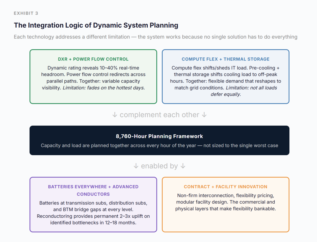
What makes this all work is looking at the full 8,760 hours in a year. Today, interconnection studies and system planning are designed around the single worst-case hour. In other words, infrastructure is sized, and costs are allocated, around a scenario that almost never actually shows up. Dynamic System Planning requires looking at every hour: understanding when the grid has headroom (most hours), when it is constrained (some hours), and when it is truly stressed (very few hours). Every technology in the portfolio is really just solving for a different part of the picture.
There’s a critical implication that the shapes of both the capacity curve and the load curve aren’t fixed. They are determined by the relative economics of flexibility investments on the grid side versus the campus side. Grid-side investments raise and flatten the capacity envelope. These include: utility-scale storage, peaker dispatch, demand response programs, advanced conductors, and power flow control. Campus-side investments raise and flatten the load profile to fill available headroom. Whether that’s in compute flexibility, behind-the-meter batteries, thermal energy storage, and/or on-site generation. These two portfolios are economic substitutes along with other dimensions. They include: speed, cost, complexity, volume, controllability, and risk allocation. If the grid side weren’t constrained and expensive, the dynamic capacity curve would be higher and flatter. This would then require less demand-side mitigation. Conversely, if campus-side flexibility is more cost-effective for a certain corridor, the grid doesn’t need to invest as heavily in reshaping its capacity profile. The reason is that compensation is better suited to the demand side.
This builds on an insight made by Arushi Sharma Frankof Luminary Strategies. As the sponsor of PGRR134, she drove the protocol design that would allow large loads to be dispatched in SCED (Security-Constrained Economic Dispatch), price nodally, and connect under a connect-and-manage framework in ERCOT. She articulates that the grid optimization problem is fundamentally about moving load and capacity across time and space. Her ERCOT work puts this into reality, where large loads are allowed to be dispatched in SCED, price nodally, and connected under a connect-and-manage framework. DSP recognizes that the relative cost of time-and-space adjustments on the electron side versus the compute side determines which portfolio yields the most value per dollar invested. The most optimal DSP portfolio for any corridor is a mix that minimizes the total system cost across both sides of the meter. That mix is different for every corridor, climate zone, load profile, and set of local grid conditions. The exhibits that follow show these curve shapes for a representative corridor. In practice, the grid side and campus side shapes are both outputs of the economic optimization, not inputs.
Filling the Headroom: The Seasonal Compute Challenge
The winter charts raise a reasonable question. If DSP reveals 500-700 MW of corridor capacity for thousands of hours per year, what compute actually fills that headroom? Data centers today do not deploy seasonal IT capacity. GPU servers amortize over 3-5 years and lose money at low utilization. A cluster that runs at 6,000 hours per year instead of 8,760 increases fixed capital cost-per-compute-hour by about 46% (on a fixed-capex basis). That’s all before any variable cost effects hit. The supporting infrastructure (cooling, power distribution, networking), is similarly capital-intensive. They can’t be economically justified at reduced duty cycles.
Seasonal hardware isn’t the solution here, but rather, it’s tiered compute tranches. These compute tranches are aligned to the corridor’s capacity duration profile. For a DSP campus, they could structure their IT deployments in layers. For instance, a firm tranche operating 8,760 hours at the corridor’s guaranteed floor capacity, running latency-sensitive workloads that require continuous availability. Another example is a shoulder tranche operating roughly 7,000-8,000 hours per year during the vast majority of hours when DXR confirms headroom above the floor. This then runs high-value AI training and batch inference. Lastly, an opportunistic tranche operating 4,000-6,000 hours during the highest-headroom periods (winter, overnight, mild weather), running deferrable workloads like model training, data processing, and pre-computation. Each tranche would be priced to reflect its expected uptime and/or duty cycle, with lower power costs for lower-firmness tranches, reflecting the non-firm interconnection structure.
The economics are challenging but not impossible. Cloud hyperscalers already sell interruptible compute at 60-90% discounts. Amazon Web Services (AWS) Spot Instances and Google Preemptible VMs are two familiar examples. These types of discounts show that there’s a market demand for lower-firmness capacity. Operators like Lancium and Crusoe have actually made this their core bet. They pair compute with variable energy sources. Within campuses, they experience the cascading lifecycle of GPU hardware. This creates a natural supply of lower-value compute that can tolerate reduced duty cycles. The key enabler is the same as everywhere else in DSP: the 8,760-hour view that makes each tranche’s expected utilization visible and contractable.
A Day in the Life
Consider a data center campus contracted at 400 MW. Under today’s planning, that is the ceiling. The campus is built to 400 MW, contracted at 400 MW, and operates at or below 400 MW every hour of the year, regardless of actual grid conditions.
Dynamic System Planning turns this whole picture on its head. That’s because both the grid side and the load side become dynamic. On the grid side, DXR is constantly recalculating to figure out the corridor’s actual thermal capacity. It does this based on real weather and loading conditions. On the load side, the campus is designed differently. It has modular capacity blocks, thermal energy storage, compute flex orchestration, and behind-the-meter batteries. They allow it to expand and contract in response to available grid capacity. The interconnection agreement reflects this. Instead of having a flat 400 MW firm contract, the campus has a dynamic capacity allocation. This provides them with the benefit of having a floor they can always rely upon. In addition, they have additional capacity that they can access whenever DXR confirms headroom.
The result: on a cold, windy January night, DXR shows the corridor has room for 520 MW. The campus activates additional modular capacity and ramps to 480 MW. It trains large AI models queued for exactly this window. On a mild spring evening, the corridor supports 500 MW, and the campus runs near that ceiling. Yet under the old static planning framework, 400 MW would have been the permanent ceiling. That includes the real capacity that was always physically available in the grid but invisible to the old planning framework.
When a hot August afternoon occurs, the corridor’s dynamic capacity shifts to its static rating. The thermal headroom may still exist, but it may run into some hiccups. Like with voltage, stability, protection, and contingency constraints, they bind independently. Any of them can set the effective limit for that hour. The corridor’s deliverable capacity holds at the contractual floor of 400 MW (the contractual floor), which the campus will respond to. The compute flex orchestration comes into effect, shifting deferable inference workloads to cooler hours or a sister facility in a different zone. Thermal energy storage is pre-cooled overnight when the grid has abundant headroom. That reduces the cooling load by 15%. Also, behind-the-meter battery storage provides another buffer. The campus holds just below 400 MW. It will never drop service that needs it the most. It rides through the stress window without curtailing below its contracted capacity, where there isn’t a reliability event needed.
This scenario rests on several conditions that must be designed in from the start, not retrofitted later. DXR forecasts must be available when campuses need them. Ramp rates for modular capacity must be fast enough to respond within the forecast window. In addition, battery duration must cover the full constrained period. Thermal energy must also be sized to expected peak stress windows (not average conditions). Curtailment notice periods must be clearly defined and agreed with the utility in advance. Lastly, when the load is shifted to a sister facility, that facility must have confirmed headroom to absorb it. None of these are deeply challenging, but each presents a design and contractual requirement.
Now layer in the commercial structure. The campus holds a non-firm or flexible interconnection agreement. This allows the campus to draw above 400 MW when DXR confirms headroom. This is all the while committing to curtail below 400 MW during the few truly constrained hours per year (extreme conditions beyond those shown in the illustrative charts). This flexibility is priced into the rate, lowering the campus’s all-in power cost below what a fully firm 400 MW customer pays. And the advanced conductors recently installed on the tightest section of the corridor (reconductored in months rather than years a new line would take) provide a permanent 30% uplift that raises the baseline for the next stress event.
The Core Technologies
Dynamic Rating (DXR)
The industry has historically used separate terms for dynamic ratings on different equipment: DLR for dynamic line rating, DTR for dynamic transformer rating, and DCR for dynamic cable rating. This paper uses DXR as a unifying term.
Dynamic rating’s evidence base varies meaningfully by asset class. For overhead transmission lines, where capacity uplift of 10-30% on average across the year is well-documented, with significantly higher gains on optimal days such as cold, windy winter conditions in Nordic climates. Transformers, cables, and other corridor elements respond more slowly to ambient conditions and have a less mature evidence base for dynamic rating, though they represent a real and meaningful source of additional headroom. The full-chain DXR concept extends this logic across every element in the delivery path; the corridor-level uplift will reflect the mix of equipment involved and which element is binding in any given hour.
A key enabler is the approach taken by companies like ATO Energy, whose platform can operate without requiring the installation of new dedicated sensors on every line or asset as a prerequisite. Sensorless in this context does not mean anti-sensor; it means the platform can use existing utility data, including any sensor data already in place, and does not need new dedicated hardware to get started. It uses weather data, grid topology, and thermal models to calculate dynamic ratings from what utilities already have. This dramatically lowers the barrier to DLR adoption, since utilities do not need to commit to a hardware deployment program before they can begin generating dynamic ratings.
Machine learning is accelerating this further. ML-enhanced weather forecasting and temporal convolutional networks can predict thermal capacity hours ahead with greater accuracy than physics. These types of models give grid operators the advanced visibility they need to make operational decisions based on dynamic ratings rather than reacting in real-time. But dynamic rating is not simply a software deployment. While the analytical capability can be stood up quickly, the implementation requires integrating DXR outputs into operational processes, rerunning system studies under dynamic assumptions, and establishing the protocols by which dynamically-rated capacities are assigned to loads and updated in real-time. This is a planning and operational transformation, not just a software license. It’s one that takes deliberate effort to implement, but on a timeline of months to a couple of years, not the decade required for new transmission.
There is a critical limitation. That is, the dynamic rating is not very effective on extremely hot, still days, when the grid is the most stressed. This is precisely why DLR is insufficient on its own and has to be paired with demand-side flexibility. The technology reveals the headroom, while the portfolio manages what happens when the headroom disappears.
Dynamic rating also introduces a question that static ratings avoid: what happens when the calculated capacity is wrong? Static planning has always had a built-in cushion. Their worst-case ratings quietly absorb whatever the forecast gets wrong. On the other hand, in a dynamic world, that margin must be explicitly designed in. DXR providers address this through conservative bias in their thermal models. The reported capacity is typically set below the true calculated limit, ensuring that any error falls on the safe side. DSP’s demand-side flexibility provides a second layer of protection: if DXR capacity drops unexpectedly, compute flex and battery dispatch respond in real-time to bring load below the revised limit. But the liability framework remains unsettled. Utilities will need a clear allocation of responsibility between different roles. They include DXR providers (for rating accuracy), grid operators (for operational decisions), and load operators (for curtailment compliance) before dynamic ratings can be used in binding interconnection agreements. This is a solvable institutional problem, not a technical one, but it must be solved.
Compute Flexibility
Compute flexibility shifts, shapes, or sheds data center electrical load in response to grid signals (price, frequency, and capacity constraints). Mechanisms include workload migration between facilities, deferral of batch and training jobs, inference load modulation, and pre-computation during off-peak hours. Tyler Norris’s research at Nicholas Institute for Energy, Environment & Sustainability suggests that data center demand-side flexibility could unlock 76+ GW of effective grid capacity nationally at just 0.25% annual curtailment, and closer to 100 GW at modestly higher flexibility levels, without new transmission. These figures represent a national potential ceiling; realized flexibility in any given case will depend on workload class, contractual structure, and how the facility was designed to operate.
The biggest challenge comes down to the operation. Compute flex requires certain workload-level visibility and orchestration tooling that most operators don’t have at scale yet. It must be remembered that not all workloads are equally deferrable. Like latency-sensitive enterprise AI inference, it should be treated very differently from batch model training. There needs to be some standardized frameworks for defining notification periods, ramp rates, and event duration. EPRI’s Mosaic initiative is a good start with this.
This aligns much with what dynamic rating is. When DXR shows the grid has headroom, compute flex ramps up. When DXR sees the grid tighten, compute flex pulls back in response. This creates a feedback loop that neither technology can achieve alone. In practice, this means AI-driven orchestration tools are handling multiple job queues at the same time. Operators measure them against real-time DXR signals, power prices, and workload priority. They are the connective tissue that makes this feedback loop operate at the speed and scale required. Early pilots have demonstrated meaningful cost reductions through AI-driven demand response in data centers; as DXR data feeds become standard inputs to these systems, the optimization becomes more precise, and the value of flexibility becomes fully capturable.
Thermal Energy Storage and Pre-Cooling
Cooling is the largest non-IT load in a data center. It is often 30-40% of total facility power in conventional air-cooled facilities. It’s important to point out that this fraction is declining. Liquid cooling adoption is a reason why, as it accelerates for AI workloads. Thermal energy storage plays an important part, allowing the cooling load to be decoupled from the hours it’s consumed. This includes things like ice systems, chilled water tanks, or phase-change materials. The facility will then pre-cool overnight or when off-peak times come about. They do this as the grid has abundant headroom, and DXR shows high capacity during those times. It will then draw down stored cooling when the constrained afternoon peak occurs. When this happens, the effect is a direct, noticeable shift of MW from peak to off-peak. It’s not a reduction in service, but a time shift of the energy required to deliver it.
This is exactly what infrastructure-level flexibility is. Where there are no workloads that are deferred, no compute curtailed, and the IT environment is unaffected. That distinction matters. Compute flexibility requires coordination with application owners and workload schedulers. Thermal storage requires only mechanical systems and control logic. It is the most operationally simple flexibility asset in the portfolio. A 100 MW campus with roughly 35 of cooling load can shift around 15-20 MW from a four-to-six hour afternoon peak to the overnight trough, every day. This all doesn’t have an impact on IT operations. When looking in purely energy terms, that is about 60-120 MWh of thermal load shifted each day. For an exact figure, it all depends on the cooling architecture, storage duration, and operating strategy. The simple constraint here is duration. Ice and chilled water systems typically provide 4-8 hours of stored cooling before requiring recharge. This is well matched to the afternoon peak stress window. It may not fully cover multi-day heat events, though, without supplemental strategies.
Battery Storage, Everywhere
Batteries are the universal bridge in Dynamic System Planning, and their value multiplies when deployed at every level of the system. At transmission substations, grid-scale batteries absorb congestion and provide fast frequency response. At distribution substations, they buffer the local delivery path and reduce transformer stress. Behind the meter at the data center campus, they cover latency-sensitive loads during the few hours when DXR shows the corridor truly constrained, and compute flex alone cannot solve the gap. Battery costs continue to decline (installed utility-scale BESS systems range from $150-300+/kWh depending on configuration, scale, and geography, with costs continuing to decline), and value stacking across congestion relief, frequency regulation, capacity reserves, and non-firm interconnection backup improves the return on investment at every deployment tier.
The strategic framing is “Bring Your Own Flexibility”. This replaces the traditional Bring Your Own Power model with on-site and grid-adjacent flexibility assets that benefit the operator and the grid. The operator can achieve lower costs and faster interconnection; the grid then experiences reduced peak stress and improved controllability.
Advanced Power Flow Control
Advanced power flow control devices play an important role. They redirect electricity across parallel transmission paths to reduce congestion and unlock capacity on constrained corridors. These devices include phase-shifting transformers, static series compensators, and power flow controllers. They create a single overloaded line bottleneck, while parallel paths run underutilized. Power flow control rebalances the system without building anything new. Combined with DXR, this creates a supply-side optimization layer. DXR reveals the true thermal capacity of each path. Power flow control routes power to exploit that capacity most efficiently.
Advanced Conductors
Reconductoring existing transmission corridors with high-temperature, low-sag (HTLS) conductors provides 2-3x the current rating on the same towers and rights-of-way. Timeline and uplift are corridor-dependent, but reconductoring is consistently faster than new build. Well-positioned corridors have been completed in as little as six months. More broader or more complex deployments typically run 12-18 months, compared to 7-12 years for new transmission.
The synergy with dynamic rating is one that goes from diagnostic to investment. DXR data identifies which corridors are most frequently constrained and would benefit most from permanent capacity upgrades. Instead of reconductoring based on static studies and political negotiation, investment follows operational data.
Contract and Facility Innovation
The commercial layer makes the portfolio economically worthwhile. Under today’s static planning, a campus is capped at 400 MW (the worst-case corridor rating). They must also contract for firm service at that level. Under DSP, the same campus could hold a non-firm agreement that allows it to operate above 400 MW when DXR confirms headroom. This is while committing to curtail during the 50-100 truly constrained hours per year. The campus gets more effective capacity from the same corridor. The utility gets a controllable, predictable load. Non-firm interconnection agreements, interruptible large-load tariffs, and conditional use arrangements that are tied to real-time grid conditions are still rare (with Texas making the most progress). Outside of Texas, what’s missing is a planning framework that makes the value visible. As well as operational tooling that makes them reliable.
Flexibility must be physically designed on the facility level. That includes: modular power and cooling capacity, thermal energy storage, adaptive cooling strategies, and on-site generation as a dispatchable resource. You cannot offer what you cannot physically deliver.
The Role of AI, and a Note on Quantum
Artificial intelligence is an enabler at every layer. ML-based thermal models extend DXR accuracy and improve forecasting. With reinforcement learning agents, they optimize workload based on scheduling on real-time grid signals. AI-powered digital twins of transmission corridors can simulate the 8,760-hour interactions between dynamic ratings, load flexibility, and storage dispatch that would take conventional power flow tools orders of magnitude longer to compute. This makes the full-year studies DSP computationally practical. Graph neural networks are being developed as surrogate models for optimal power flow analysis, potentially compressing what today’s multi-hour study runs into minutes. Things like predictive maintenance algorithms, trained on transformer and cable sensor data, can forecast equipment degradation and adjust dynamic ratings before failures occur.
This is not speculative. ThinkLabs AI, a physics-informed AI company backed by NVentures (NVIDIA‘s venture capital arm) and Edison International, has demonstrated the ability to compress a month-long grid engineering study into under three minutes, running 10 million power flow scenarios in 10 minutes at greater than 99.7% accuracy (per Thinklabs’ published reports). In collaboration with Southern California Edison (SCE), ThinkLabs’ ML models trained in minutes per circuit, processed a full year of hourly power-flow data across more than 100 circuits, and produced bridging-solution recommendations with engineering reports in under 90 seconds. Traditional utility engineers spend an average of six hours per project preparing data, running power flow, and generating reports, with full energization analyses requiring 30-35 days. ThinkLabs’ approach collapses this by orders of magnitude. For DSP, the implication is quite direct. The computational objection to 8,760-hour studies is no longer credible. Physics-informed AI digital twins can run the full-year, multi-scenario analyses that Dynamic System Planning requires. It does this at a speed and cost that makes them routine rather than exceptional.
Quantum computing and quantum sensing are things to look for in the future. With quantum optimization algorithms (quantum annealing, variational methods), they show theoretical promise for the combined problems at the heart of grid planning. This includes: unit commitment, optimal power flow, and the 8,760-hour scheduling problems that DSP introduces. Practical quantum advantage for these problems is likely 7-15 years away, limited by qubit error rates and coherence times. Quantum sensing could further improve DXR accuracy beyond what classical sensors achieve. The practical benefit over current sensor technology (already accurate to ±2°C) may be marginal, though. These are technologies to track, not to depend on. DSP is designed to work with today’s tools; AI and quantum will make it work better.
The Economics
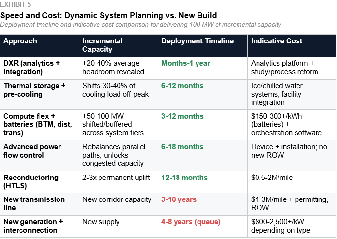
The economic case rests on three pillars. First, speed: DXR plus compute flex can unlock interconnection capacity in weeks to months, not years. Reconductoring delivers permanent uplift in 12 –18 months. Contract innovation can move projects through the interconnection queue faster by reducing the firm capacity requirement. For a data center operator facing a five-year queue, a portfolio that delivers 80% of the capacity in six months at 60% of the cost isn’t a compromise. It’s a competitive advantage.
The second is centered on cost. Unlocking 20-30% more capacity from existing transmission through DXR analytics and study process reform compares favorably to $1-3M per mile for new transmission. This avoids expensive and multi-year construction of new substations along with their long-lead equipment, as well as transmission, which can get caught up in regulatory, permitting, and right-of-way processes.
Third, reliability: a portfolio approach actually reduces single-point-of-failure risk. Grid operators gain real-time visibility and controllability over large loads, a better outcome than the current model, where a large firm load is a black box behind the meter. But the question is no longer whether dynamic operation is conceptually compatible with reliability requirements. It is whether utilities are ready to study, trust, and operationalize it. That requires more than a dynamic rating output. Utilities will need to understand how large loads behave during voltage disturbances, whether protection and control systems are properly coordinated under dynamic conditions, how behind-the-meter batteries and load controls interact with utility systems, and whether asset and load behavior is modeled with enough fidelity for planning and contingency analysis. This is where ATO's role extends beyond revealing dynamic headroom. Their platform can support the surrounding reliability analysis that utilities will require before they rely on dynamic operation at scale, helping bridge the gap between technical capability and operational confidence. Flexibility isn't a concession; it is an edge for operators who embrace it..
What Needs to Change
The Single-Worst-Hour Problem
The most fundamental barrier is how the grid is studied and planned today. System studies, interconnection analyses, and engineering assessments are built around the single worst-case condition, typically a handful of peak hours per year. Every component is sized, every rating is set, and every cost is allocated as if that worst hour is the only hour that matters. This methodology ignores the 8,700+ hours where the grid has significant headroom, makes it impossible to value load shifting or curtailment commitments, forces all interconnecting loads to be treated as firm 24/7 worst-case consumers, and renders the entire Dynamic System Planning approach invisible to the planning process.
Until system studies move to an 8,760-hour (or at a minimum, probabilistic and multi-scenario) framework that accounts for hourly variation in both grid capacity and load, the value of these solutions cannot be captured in interconnection agreements, tariffs, or investment decisions. This is the single biggest unlock, and the single biggest blocker. The computational excuse is fading, though. As brought up earlier, AI platforms (like ThinkLabs AI) have demonstrated their effectiveness already. Their results are demonstrated in research and pilot scenarios, with production deployment in RTO planning workflows still nascent. The barrier is institutional, not technical.
Regulatory and Institutional Inertia
Many US jurisdictions still do not accept dynamic ratings for planning purposes (with ERCOT being a notable exception). Federal Energy Regulatory Commission and state PUCs default to static thermal limits. FERC Order 2023 improves the interconnection queue process, but it doesn’t change the worst-case study methodology. And utilities have limited incentive to adopt dynamic ratings that reveal their existing lines have been underutilized for decades.
Commercial Misalignment
Data center operators contract firm capacity as a reliability hedge. Utilities price firm service as a revenue guarantee. Neither side has strong incentives to move to flexible arrangements today. Non-firm or interruptible large-load tariffs exist in theory but are rarely structured to make flexibility economically attractive.
Technology and Operational Gaps
Compute flex orchestration is nascent. DXR requires grid data sharing between TSOs and technology providers; compute flex requires operators to share load profiles. They both face data governance and competitive sensitivity barriers, though. And no common framework yet exists for defining, measuring, and verifying flexibility contributions from large loads, though EPRI’s DCFlex initiative and Mosaic standards are important early steps.
Cybersecurity and Data Sharing
Dynamic System Planning depends on real-time or near-real-time data flows between grid operators and load operators: DXR outputs from TSOs to campus operators, load profiles from campuses to grid planners, and dispatch signals in both directions. This creates cybersecurity exposure that does not exist in today’s static planning model. Who has access to dynamic rating data? Who bears liability if a dynamic rating is wrong and a thermal limit is exceeded? How are load profiles protected from competitive disclosure? These questions do not have settled answers. They will require things like new data governance frameworks, secure communication protocols, and clear liability allocation, all before DSP can operate at scale.
Extended Stress Events
The flexibility portfolio is well-suited to managing the grid’s typical stress pattern. There’s a handful of peak hours on hot afternoons, bookended by overnight recovery. But climate change is making multi-day heat events more frequent. There are extended heat domes where high temperatures persist for five to seven consecutive days with limited overnight cooling. Under these conditions, hurdles might arise. Whether it be thermal storage not fully charging overnight, battery reserves depleting across consecutive discharge cycles, and DXR showing sustained constraint rather than intermittent stress, the portfolio is designed to manage. DSP must be honest about this boundary. For multi-day extreme events, the portfolio buys time and reduces severity, but it doesn’t eliminate the need for firm capacity reserves or new infrastructure. The long-term buildout remains essential; DSP accelerates what is possible in the interim.
DSP for Generation and Storage Interconnection
The data center load case is where DSP’s value is most immediate, but Dynamic System Planning applies with equal force to the other side of the interconnection queue: generation and storage. The 2,300+ GW backlog waiting to connect is not just data centers. It is also in solar farms, wind projects, gas peakers, and battery storage facilities. With them all experiencing the same single worst hour study methodology, as well as the same static planning bottleneck.
Consider solar generation. A solar farm’s output is inherently variable, producing power only when the sun shines, with a capacity factor of 20–30% in most regions. Yet the interconnection study evaluates its impact on the grid at peak output under worst-case system conditions and sizes the required network upgrades to that single scenario. The DXR correlation that benefits wind (cold and windy conditions boosting both output and line capacity simultaneously) does not apply as cleanly to solar: peak solar output coincides with hot afternoons when ambient-cooled transmission lines are at or near their thermal limits. DXR alone may not unlock significant additional headroom during the hours that matter most for solar interconnection. But the 8,760-hour study framework still transforms the analysis. Solar output occurs across thousands of hours with widely varying grid conditions, and an hourly evaluation reveals that the worst-case injection scenario (peak output into a fully loaded grid on the hottest day) occurs only a handful of times per year. For the vast majority of production hours, the grid can absorb the output without upgrades. Pairing solar with co-located or grid-adjacent battery storage (the “BESS everywhere” approach) completes the picture: batteries absorb injection during the few constrained hours, shift delivery to periods when the grid has headroom, and allow the solar farm to interconnect faster, at lower cost, with a smaller upgrade footprint.
Wind generation benefits even more directly. Wind output is highest when conditions are cold and windy, exactly the conditions that maximize dynamic transmission capacity. A study taking DXR into account would show that the corridor’s capacity to absorb wind generation is highest when the wind is blowing hardest. That dramatically reduces the curtailment risk and upgrade costs that static studies assign.
Gas generation and storage interconnection face a similar dynamic as well. For example, a gas peaker that runs 500-1,000 hours per year during peak demand is studied as if it injects full output under worse-case grid conditions. This happens even though the grid’s capacity to absorb that injection varies immensely across those hours. Battery storage is doubly penalized by static studies. They evaluate both the charge and discharge scenarios in their worst cases. This is all instead of optimizing across the 8,760-hour dispatch profile.
The implication is very significant. Dynamic System Planning could block capacity for generation and storage interconnection just as it does for load. It compresses timelines and reduces upgrade costs across the entire queue. The same 8,760-hour framework, the same DXR visibility, and the same principle all apply. This is true regardless of whether the interconnecting resource is consuming or producing power.
The framework goes even further. Electrification is adding tens of gigawatts of new load that shares the same characteristic as data center demand: it is flexible if the planning process can see and value that flexibility. EV fleets, networked water heaters, smart thermostats, and building energy management systems can all play a big part. They can all curtail, shift, or modulate in response to grid conditions. These distributed loads act as a demand side resource that DSP’s 8,760-hour framework can integrate alongside large industrial flexibility. The planning methodology stays the same as well. Dynamic supply visibility on one side, classified, and contracted flexibility on the other, optimized across every hour of the year. The scale of the individual resource differs; the planning logic does not.
Building on the Momentum, and Why Dynamic System Planning is Different
This paper is not the first to challenge static grid planning. The intellectual groundwork is being laid across several fronts, each important, each incomplete on its own.
Tyler Norris’s research at Duke University (“Rethinking Load Growth”) helps build on this narrative. It found that the US power system could accommodate 76+ GW of new load if those loads provide just 0.25% flexibility. His core finding is that the average system load factor is roughly 53%. That means half of the generation and transmission capacity sits unused in any given hour. This is a powerful indictment of the status quo, but Norris’s framework addresses the demand side in isolation. The grid is treated as a fixed constraint that loads flex around.
The WATT Coalition has been the main advocacy voice for Grid Enhancing Technologies (GETs) in transmission planning. They are supported by the economic analysis from The Brattle Group. Their work demonstrates that DLR, advanced power flow control, and advanced conductors can defer or reduce the need for new transmission buildouts. For example, with PPL Electric Utilities’ DLR deployment in Pennsylvania, it reduced congestion costs by over $60M per year on a single line. GETs still focuses on supply-side uplift capacity, though. They do this without deeply integrating demand-side response, which makes that uplift bankable.
FERC has begun codifying the shift. Order 881 (2021) mandates ambient adjusted ratings, which is a step towards dynamic ratings. Three years later, Order 1920 (2024) required transmission planners to consider DLR, advanced conductors, and power flow control in long-term planning. The implementation is lagging, though. Most transmission providers have sought extensions beyond the original June 2025 compliance deadline. The first long-term planning cycles under Order 1920 may not happen until 2027-2028. The regulatory architecture is moving in the right direction, but at a speed that doesn’t match the urgency of load growth. In addition, it still treats supply and demand in separate proceedings.
EPRI’s DCFlex initiative, launched in late 2024 and now comprising over 65 participants, is the most direct parallel effort. It includes some big names like Google, Meta, Nvidia, and several major utilities. The Flex MOSAIC workstream establishes a common language for characteristic data center flexibility. It includes: notification periods, ramp rates, and event duration. Another workstream is looking to incorporate that flexibility into grid planning and interconnection processes. This is important foundational work, but DCFlex is primarily a classification and standards effort. It doesn’t yet propose an integrated planning methodology that couples supply-side dynamic visibility with demand-side flexibility across the full 8,760 hours. It also doesn’t address how DXR-revealed headroom and load flexibility should be co-optimized in interconnection studies. DSP builds on the standardization DCFlex provides and extends it into a complete planning framework. The two are designed to be complementary: a campus whose flexibility is classified using MOSAIC metrics can have that classification directly incorporated into a DSP-based interconnection study, connecting the common language DCFlex creates to the planning methodology that puts it to work.
The proof-of-concept is accelerating in real-time. In October 2025, PJM, Nvidia, EPRI, Digital Realty, and Emerald AI announced the Aurora AI factory in Manassas, Virginia. It will be a 96 MW facility designed as a power-flexible AI infrastructure. It will be the first built to a new reference design and certification standard for flexible large loads. The facility deploys Emerald AI’s Conductor platform as its grid-orchestration layer, integrated with Nvidia’s DSX Flex library, which provides GPU-level power telemetry at seconds granularity, enabling the facility to ramp power up or down in real-time in response to grid signals. In March 2026, Emerald AI closed a $25 million strategic round (also backed by NVentures, alongside Eaton, GE Vernova, Siemens, and others), and Nvidia and Emerald jointly estimated that if the power-flexible AI factory reference design were adopted nationwide, it could unlock up to 100 GW of capacity on the existing US electricity system. On that same day, ThinkLabs AI closed a $28 million Series A. It was also led by Energy Impact Partners, also backed by NVentures (Nvidia’s venture arm), the same pairing behind the Emerald round. Together, the two rounds raised a combined $53M across grid-side intelligence (ThinkLabs) and demand-side orchestration (Emerald) in a single day. It’s a signal that the industry’s most consequential infrastructure company views both sides of the DSP equation as essential.
A 2025 Nature Energy paper, “AI data centres as grid-interactive assets,” demonstrated a software-based approach on a 256-GPU cluster in a hyperscale facility in Phoenix, achieving a 25% power reduction during a three-hour peak demand window while maintaining AI quality-of-service guarantees, with no hardware modifications or on-site storage required. Google has demonstrated temporal and spatial workload shifting across its global data center fleet. These examples confirm that the demand-side flexibility DSP assumes is not theoretical; it is being built, funded, and tested at scale. What is missing is the planning framework to harness it systematically.
DSP is a complement to long-term grid buildout, not a replacement for it. Firm capacity still matters; not every large load will or should become interruptible, and dynamic ratings alone do not solve adequacy, congestion, or interconnection bottlenecks. New infrastructure will still be required. The point of DSP is to extract more from what exists, identify where flexibility can credibly substitute for or defer upgrades, and improve how technical headroom is translated into planning decisions.
Dynamic ratings exist. Flexible loads exist. What does not yet exist is a planning framework that integrates both sides across every hour of the year. That is what Dynamic System Planning provides.
Each of these threads addresses a piece of the puzzle: Norris argues for flex loads, WATT advocates for GETs, Brattle models the economics, FERC sets the regulatory floor, EPRI’s DCFlex builds the standards, and hyperscalers prove the demand-side mechanics work. Dynamic System Planning is the integration layer. It’s a framework that connects all of these into a single operational planning methodology where the grid’s capacity and the load’s flexibility are planned together, across 8,760 hours, as a coupled system.
This means dynamic supply visibility (DXR) and dynamic demand response (compute flex, storage, shifting) are coordinated in a single planning model. It’s not siloed in separate interconnection studies and demand response programs. This means the planning horizon is 8,760 hours. That enables the system to value things like curtailment commitments, shifting capabilities, and variable capacity in interconnection agreements. Permanent infrastructure investment (advanced conductors, storage) is then targeted by diagnostic data from dynamic operations. DXR identifies the bottleneck, compute flex quantifies how often it binds, and the investment case writes itself. It also means commercial structures emerge naturally from the 8,760-hour view. That’s because the value of flexibility is finally visible and measurable.
Dynamic System Planning is not a new technology. It is a new way of planning around the technologies that already exist.
The Path Forward
Dynamic System Planning does not require waiting for new technology, new regulation, or new consensus. Every component exists today, but what’s needed is a structured sequence of actions that brings them together.
Near-Term (Next 12 Months): Prove It on a Real Corridor
A single pilot project is the most important next step. One where a utility, data center developer, and DXR provider get together and run an 8,760-hour study on a corridor that’s being squeezed. They’d deploy dynamic ratings, model actual load flexibility, and put a number on how much capacity the combination actually frees up. The latter being something a static study never could. This pilot should be jointly published with full methodology and results. That then gives the industry its first empirical reference point for DSP.
The output should not simply be “capacity varies hour to hour.” It should be decision-grade: what capacity can credibly be treated as firm, what can be conditional or flexible, what hours or conditions bind, what operating commitments are required, and what targeted upgrades or fallback measures still remain necessary. We (impactECI) are actively pursuing this with partners.
Grid operators and ISOs should begin running parallel 8,760-hour analyses alongside existing worst-case studies on selected corridors, not as replacements, but as proof-of-concept comparisons. The computational tools exist; the incremental cost is software, not steel. PJM or MISO would be ideal first movers, given their acute load growth pressure.
Medium-Term (12-14 Months): Build the Commercial Framework
Data center operators need to get serious about compute flex tooling, facility-level flexibility assets, and operational discipline to back it up. This offers credible curtailment and shifting commitments. The operators who demonstrate EPRI DCFlex-classified profiles and pair them with DXR-informed interconnection requests will get through the queues faster and cheaper than those demanding fully firm service.
Regulators (FERC, state PUCs) should speed up the implementation of Order 1920. They should also close the gap between the supply side (GETs in planning) and the demand side (flexible interconnection) proceedings. Specifically, FERC should give some guidance on how non-firm interconnection agreements tied to real-time dynamic ratings can satisfy reliability requirements. Also, state PUCs should pilot interruptible large-load tariffs with pricing indexed to DXR-revealed capacity. The U.S. Department of Energy (DOE) SPARK program put $1.9 billion behind exactly the supply-side half of this stack. There are explicit thresholds for DLR deployment and reconductoring as well. Regulators and utilities should take advantage of this and position themselves to get this support.
PJM, MISO, CAISO, and NYISO should all evaluate protocol revisions to their own market structures. ERCOT has already demonstrated the template, but the question is whether there is institutional will to use it.
Longer-Term (24+ Months): Institutionalize
Technology providers must pursue interoperability standards. This means DXR platforms, compute orchestration systems, and battery management systems need a common real-time data protocol. The DSP portfolio can then be operated as a coordinated system, not a collection of independent tools. AI-powered digital twins and ML surrogate models for power flow analysis should be developed specifically for 8,760-hour DSP studies, reducing computational barriers to full-year planning.
The industry must build off the pilot results, developing standardized DSP study methodologies that RTOs and utilities can adopt. EPRI’s DCFlex initiative is the natural convening body; DSP provides the integrated planning framework that DCFlex’s flexibility standards can plug into. As this paper goes to press, EPRI has formally launched Flex MOSAIC at CERAWeek 2026, establishing the common flexibility classification language that DSP’s planning methodology can operationalize. It’s a significant step toward making these concepts implementable.
The national implications bear repeating. Across the US transmission system, DSP-enabled corridors could deliver 100-150 GW of additional effective capacity without new rights-of-way, compress interconnection timelines from years to months for projects willing to offer flexibility, and redirect $30-60 billion from long-lead new-build transmission toward faster, more targeted portfolio investments. For data center operators, that translates to earlier revenue, lower all-in power cost, and a competitive edge in site selection. For grid operators and regulators, it means moving the interconnection queue without waiting for steel in the ground. For the broader economy, it means the energy infrastructure for the AI buildout can arrive on the timeline the technology demands, not the timeline the current planning process dictates.
Dynamic System Planning is not a wish list. It is a synthesis of technologies and practices that already exist. The grid we need is largely the grid we already have, if we plan it as a dynamic system rather than a static worst case. The first corridor that proves it will change the conversation for every corridor after.
DSP's value is not in interesting analysis. It is in turning time-varying technical reality into something utilities, developers, operators, and investors can act on with confidence.
Peter Hans Hirschboeck is Managing Director of impactECI, an advisory firm focused on data center energy infrastructure economics. He developed the Dynamic System Planning framework as part of impactECI’s ongoing work on grid flexibility, power sourcing strategy, and large-load interconnection.
The author gratefully acknowledges Peder Falkman and the ATO Energy team for their contributions on dynamic rating technology, case data, and technical review. ATO Energy’s sensorless DXR platform provided key inputs to the dynamic rating analysis in this paper.